The local chart
The most easy chart is the canonical one: just use the original (x,y) coordinates on screen. This allows to study any finite region. Example screen output: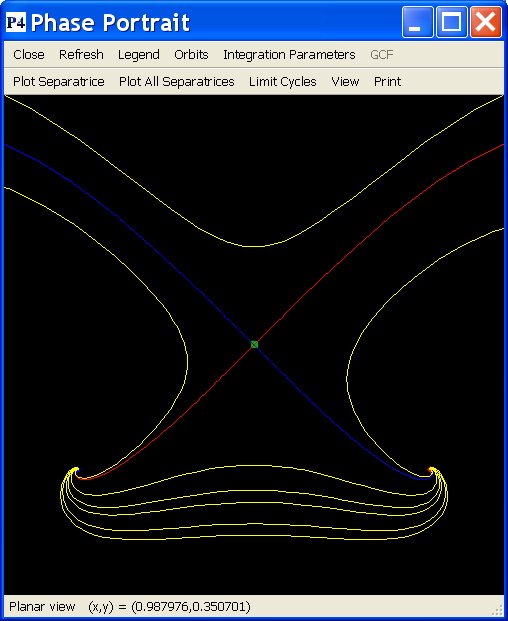
Spherical projection
Example screen output: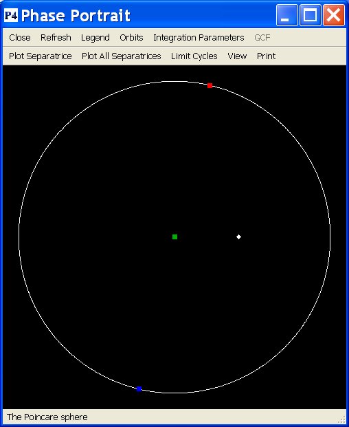
The U1 Chart
Restricting to the set Z2>0, and using the transformation { x = 1/Z2, y = Z1/Z2 } one displays a part near infinity where x is much larger than 1. In other words, one finds information near the ``eastern part of the poincare sphere''. Example screen output: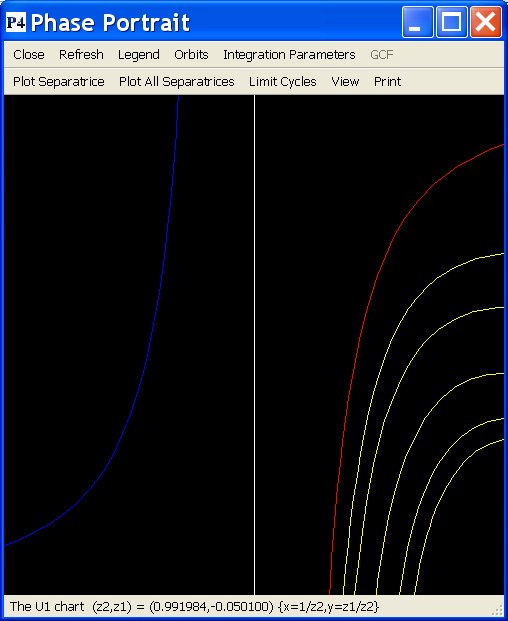
The U2 Chart
Restricting to the set Z2>0, and using the transformation { x = Z1/Z2, y = 1/Z2 } one displays a part near infinity where y is much larger than 1. In other words, one finds information near the ``northern part of the poincare sphere''. Example screen output: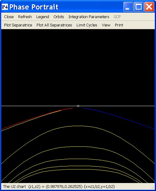
The V1 Chart
Restricting to the set Z2>0, and using the transformation { x = -1/Z2, y = Z1/Z2 } one displays a part near infinity where -x is much larger than 1. In other words, one finds information near the ``western part of the poincare sphere''. The plot axes are the (Z2,Z1)-axes. The line at infinity {Z2=0} is shown vertically in the middle, and the V1-chart is found to the right of this line. To the left, one finds the U1' chart. This U1' chart has a strong resemblence with the U1 chart but may be different, depending on the order of the vector field or the chosen Poincare-Lyapunov compactification weights.The V2 Chart
Restricting to the set Z2>0, and using the transformation { x = Z1/Z2, y = -1/Z2 } one displays a part near infinity where -y is much larger than 1. In other words, one finds information near the ``southern part of the poincare sphere''. The plot axes are the (Z1,Z2)-axes. The line at infinity {Z2=0} is shown horizontally in the middle, and the V2-chart is found on top of this line. On the bottom, one finds the U2' chart. This U2' chart has a strong resemblence with the U2 chart but may be different, depending on the order of the vector field or the chosen Poincare-Lyapunov compactification weights.Charts with Poincare-Lyapunov compactification
Example screen output for the spherical projection: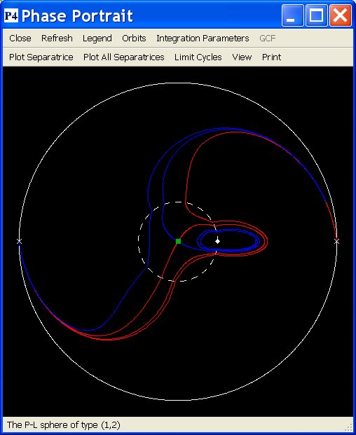
Similarities between the (U1,V1,U2,V2) and the (U1',V1',U2',V2') charts
The vector field that is studied in the charts at infinity is first desingularized: one divides by a power of Z2, related to the degree of the vector field. For that reason, when one compares the U1 with the U1' chart, it can happen that, aside from applying a reflection, the direction of integration needs to be reversed. Back to the main page